Some Econ Things
Here are some economics things I've learned, in no particular order.
This page is not remotely exhaustive of the field.
Production–possibility frontier
Andy runs a bakery. Or at least, he owns several robots that produce baked goods. Each robot can use up to \(100\) units of energy per day, the cost of which we will ignore.
Andy's menu is simple: he only sells apple pies and brownies. For the \(i\)-th robot, he knows that:
- If it uses all its energy on making apple pies, it will produce \(a_i\) of them;
- If it uses all its energy on making brownies, it will produce \(b_i\) of them.
How can Andy allocate his robots efficiently?
One robot
Let's start simple and assume Andy only has \(1\) robot. Say \(a_1 = 100\) and \(b_1 = 50\).
If the robot only makes apple pies, then it produces \(100\) apple pies and \(0\) brownies a day. We'll represent this as the point \((100, 0)\). If the robot only makes brownies, then it produces \(0\) apple pies and \(50\) brownies a day, which we'll represent as \((0, 50)\).
Of course, these are not the only two possibilities. For example, the robot can use \(50\) units of energy for apple pies and \(50\) units of energy for brownies. Then it produces \(50\) apple pies and \(25\) brownies a day, which we'll represent as \((50, 25)\). Here we're assuming that energy consumption is linearly proportional to the production of baked goods; let's not give ourselves a headache.
We can see that, if the robot uses all its energy, the set of all possibilities is represented by a straight line connecting \((0, 50)\) and \((100, 0)\). Naturally, its slope is negative; specifically it's \(-\frac{1}{2}\).
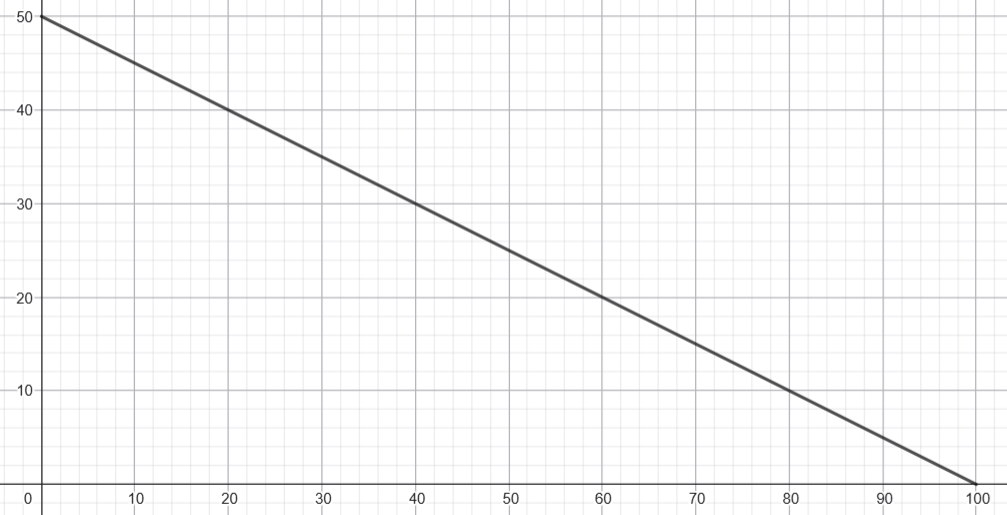
This line is called the production–possibility frontier, or PPF for short.
Here's a nice interpretation: the robot starts out at \(0\) apple pies and \(50\) brownies, and it can then "convert" \(\frac{1}{2}\) brownie into \(1\) apple pie until there are no more brownies left. Conversely, if the robot starts out at \(100\) apple pies and \(0\) brownies, it can convert \(2\) apple pies into \(1\) brownie until there are no more apple pies left.
These trade-offs are also known as the opportunity cost. The opportunity cost of \(1\) apple pie is \(\frac{1}{2}\) brownie, and the opportunity cost of \(1\) brownie is \(2\) apple pies. They are reciprocals of each other, because that's how math works.
Now, it's possible that the robot doesn't use up all its energy. For instance, if the robot uses \(20\) units of energy for apple pies and \(20\) units of energy for brownies, then it produces \(20\) apple pies and \(10\) brownies, which is the point \((20, 10)\). Unsurprisingly, this point lies below the PPF. This is clearly not efficient for Andy, assuming he only cares about producing baked goods. So from here, we'll just care about points that lie on the PPF.
Many robots
When there are multiple robots, it gets interesting, because not all robots are equally "good" at producing apple pies and brownies, for some notion of "good" we'll define shortly.
If Andy only cared about producing apple pies, then this is easy: the robots can produce \(a_1 + a_2 + \ldots + a_n\) apple pies a day. Similarly, if Andy only cared about producing brownies, then the robots can produce \(b_1 + b_2 + \ldots + b_n\) brownies a day.
But what happens in the middle? Using our conversion idea from earlier, to convert \(b_1 + b_2 + \ldots + b_n\) brownies into \(a_1 + a_2 + \ldots + a_n\) apple pies, each robot itself should gradually shift its production from brownies to apple pies. Specifically, the \(i\)-th robot gradually converts \(b_i\) brownies into \(a_i\) apple pies.
To maximize efficiency, Andy should greedily order the robots by increasing \(\frac{b_i}{a_i}\). The robot with the lowest \(\frac{b_i}{a_i}\) converts all its brownies to apple pies, then the next robot does the same, and so on, until all robots have finished their conversion.
Coming back to English, robots with a lower \(\frac{b_i}{a_i}\) are "better" at producing apple pies relative to brownies, so Andy should allocate them on apple pie duty first. To introduce some terminology, these robots have a comparative advantage in producing apple pies over other robots.
On the other hand, robots with a higher \(\frac{b_i}{a_i}\) are "worse" at producing apple pies relative to brownies, so Andy should only let them produce apple pies as a last resort, when he's run out of good apple pie producers. These robots instead have a comparative advantage in producing brownies.
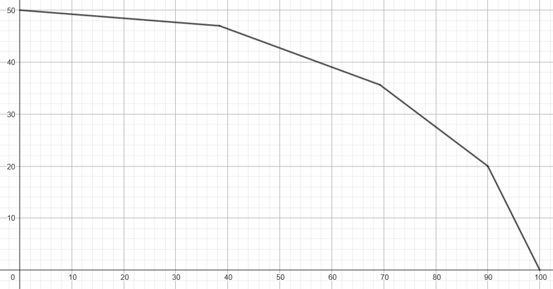
This causes the PPF to become concave: starting from the curve's \(y\)-intercept, each segment's slope decreases until it reaches the \(x\)-intercept. In more realistic models, you wouldn't necessarily have discrete segments like this; it'd just be a smooth continuous curve.
It's worth noting that, if all the robots had the same \(\frac{b_i}{a_i}\), then the PPF degenerates into a straight line as before. This is not to say that all robots perform equally well. It's just that none of them have a comparative advantage. It's entirely possible for one robot to produce more apple pies or brownies using the same amount of energy; this is called an absolute advantage.
Trading
Andy's boyfriend Benny also runs a bakery just across the road. They haven't merged yet, since they (sensibly) want to keep their relationship low-key for the time being.
We'll assume a linear PPF for both Andy and Benny. Again, if Andy's robots used all their energy on apple pies, they'd produce \(100\) apple pies a day. If they used all their energy on brownies, they'd produce \(50\) brownies a day. The corresponding numbers for Benny are \(75\) apple pies and \(45\) brownies a day. The boys just really like apple pies and brownies, don't worry about it.
Let's put everything in a table:
| Andy | Benny | |
|---|---|---|
| Apple pies | \(100\) apple pies | \(75\) apple pies |
| Brownies | \(50\) brownies | \(45\) brownies |
If Andy and Benny never interacted with each other and lived in autarky, then they could only ever hope to produce as efficiently as constrained by their respective PPFs. However, with the power of love trading, they can obtain consumption combinations outside their PPFs.
Let's now consider Andy's and Benny's respective opportunity costs:
| Andy | Benny | |
|---|---|---|
| Apple pies | \(\frac{1}{2}\) brownie | \(\frac{3}{5}\) brownie |
| Brownies | \(2\) apple pies | \(\frac{5}{3}\) apple pies |
Notice that Andy has a comparative advantage in producing apple pies, since it costs fewer brownies per apple pie. Conversely, Benny has a comparative advantage in producing brownies, since it costs fewer apple pies per brownie.
With two goods and linear PPFs, one of them should have a comparative advantage in one thing, and the other one should have a comparative advantage in the other thing. Again, that's how math works. The only exception to this is when neither has a comparative advantage over anything, but then trading wouldn't be useful anyway.
Coming back to this example, since Andy has the comparative advantage in producing apple pies, he decides to focus on only producing apple pies. Similarly, Benny decides to focus on only producing brownies.
Andy and Benny meet up at the nearest café, baked goods in hand. Andy offers \(18\) apple pies, and Benny offers \(10\) brownies. Is this a reasonable trade?
Well, the price of a trade can be expressed two ways: both from the perspective of Andy, and from the perspective of Benny. For Andy, he's converting \(18\) apple pies into \(10\) brownies, so the price of this trade is \(\frac{9}{5}\) apple pies per \(1\) brownie. This is less than if he had just used his robots to convert \(2\) apple pies into \(1\) brownie, so he's happy.
For Benny, it's basically the same thing. He's converting \(10\) brownies into \(18\) apple pies, so the price of this trade is \(\frac{5}{9}\) brownies per \(1\) apple pie. This is less than if he had just used his robots to convert \(\frac{3}{5}\) brownies into \(1\) apple pie, so he's also happy.
Mathematically, if the price of \(1\) apple pie is between \(\frac{1}{2}\) and \(\frac{3}{5}\) brownie, then both sides are happy. Similarly, if the price of \(1\) brownie is between \(\frac{5}{3}\) and \(2\) apple pies, then both sides are happy. In the end, both boys have achieved a consumption combination outside their respective PPFs.
Note that Andy has an absolute advantage over Benny in both apple pies and brownies (Benny gets teased relentlessly over this). However, it is ultimately still worth it for both sides to trade.
Market price
Of course, no bakery is without customers, so let's not forget about them.
How should Andy and Benny price their items, say, their brownies? First of all, they are competitors in close proximity (or at least, that's what the public thinks), so they should sell brownies at roughly the same price. If Andy's brownies were way more expensive, then people would flock over to Benny's bakery to get their brownie fix instead, and vice versa.
But that's in relation to each other. How should they even decide the price in the first place? Well, with… more relations. Andy has some baker friends whom he can ask how much they sell their brownies for at their bakeries. Likewise, Benny has some baker exes enemies whom he spies on with the help of Andy. And of course, there's the wonderful Internet. Just look up brownie prices and there you go.
The point is, all these prices from all these sources should (more or less) converge1. Andy and Benny can sniff around nearby bakeries, but so can the customers. If the two boys set their price too high, then people would flock over to other bakeries. If they unnecessarily set it too low, then they might be shooting themselves in the foot: customers are willing to pay more, so why should they charge less?
Now, there are some nuances to this. For example, if Andy and Benny's bakeries were right by a college campus, maybe they'd be incentivized to lower their prices just a bit for hungry students. Or maybe Benny can make his brownies a little bit more expensive, since they have chocolate chips after all. But anyway, we will forget all of that for now and assume that everything really does converge to a universal, mystical number known as the market price.
Marginal cost
As we've seen with the PPFs, the more brownies the boys produce, the more apple pies they have to give up per \(1\) brownie. This is generally true not just relative to apple pies: the more brownies you produce, the marginal cost (say, in dollars) of producing \(1\) additional brownie eventually increases. Here we'll just assume it always increases.
As a reminder, the boys are producing brownies on a daily basis, and hence we're implicitly taking the marginal cost to refer to the additional production cost of \(1\) more brownie within the same day.
Supply and Demand
Supply curve
Suppose the boys sell brownies at a market price of \(P = 3\) per brownie. Then what is the total quantity of brownies, \(Q\), that they should produce in a day? Well, the idea is straightforward. Keep producing brownies until the marginal cost of \(1\) more brownie exceeds \(3\). Say \(Q = 50\).
Now, imagine a universe where the price of a brownie is \(P = 4\) instead. Andy and Benny are smart boys, so they can run the computations and predict that in this universe, they would produce \(Q = 60\) brownies a day. Naturally, this number should be higher, since the marginal cost cut-off is now higher.
On the other hand, the boys predict that if they were in a universe where the price of a brownie is \(P = 2\), they would only produce \(Q = 40\) brownies a day. Now the cut-off is lower, so naturally, fewer brownies.
We can plot this for all possible prices \(P\) to obtain the supply curve. Well, I say curve, but you know we're only going to deal with lines. Also, unlike how you'd normally plot dependent variables, \(P\) is on the \(y\)-axis and \(Q\) is on the \(x\)-axis, because economists are funny.
Demand curve
Cindy is a good friend of Andy and Benny and a regular at their bakeries. She has quite the sweet tooth, so she finds herself craving \(1\) brownie about every \(5\) days. Using stronger (and unfortunately more common) terminology, we'll say she demands \(1\) brownie every \(5\) days, or \(0.2\) brownies a day. If the market price were higher, maybe she'd find herself wanting to buy fewer brownies (so her wallet wouldn't hurt as much). If the market price were lower, maybe she'd rejoice and find herself wanting to buy more brownies.
Of course, Cindy isn't the only customer at the boys' bakeries. We can sum up the quantities demanded across all customers for a fixed market price \(P = 3\) and call it \(Q\). Naming collision, oops. But this works out nicely, because \(Q\) coincidentally (not really lol) also happens to be \(50\).
Same idea as the supply curve, though this should be more intuitive. In a universe with a lower market price, customers would want to buy more brownies, and in a universe with a higher market price, customers would want to buy fewer brownies.
Market equilibrium
We know the supply curve has a positive slope and the demand curve has a negative slope. The point at which they intersect is the market equilibrium. Specifically, the \(y\)-coordinate, \(P\), is the equilibrium price, and the \(x\)-coordinate, \(Q\), is simultaneously the quantity supplied by the producers (the lover boys) and the quantity demanded by the consumers (the customers).
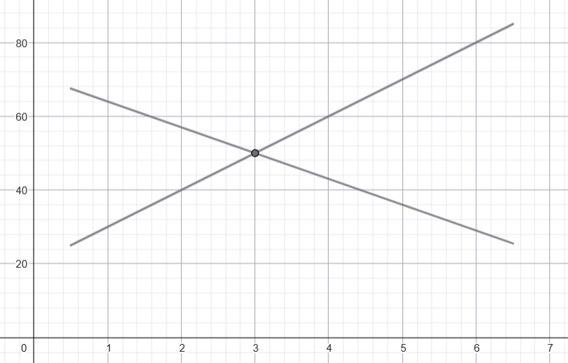
It should be emphasized that most stable markets should already be close to equilibrium. However, for the sake of exposition, let's assume we're observing the market right after a significant change.
If the current market price is higher than the equilibrium price, then there is a surplus: the boys are producing more brownies than customers actually want to buy. This is wasteful, so they'll want to decrease the price, both to produce fewer brownies, and also to encourage customers to buy more.
If the current market price is lower than the equilibrium price, then there is a shortage: the boys aren't producing as many brownies as the customers want to buy. The customers are sad and brownie-less, so the boys will want to increase the price, which incentivizes them to produce more brownies, and also helps stop Cindy from buying brownies all the time.
Shifting the supply curve
The local grocery store where Andy and Benny buy their brownie ingredients is having a massive sale! The boys are overjoyed.
The supply curve shifts to the right, because the boys can produce so many more brownies now. The demand curve stays still, since the customers are (mostly) indifferent to the boys' shenanigans. The equilibrium price goes down, because brownies are now cheaper to produce. The equilibrium quantity goes up, as customers are encouraged to buy more brownies at the lower price.
However, all good things must come to an end. The store's sale is over, and production is back to normal. The supply curve shifts to the left, so the equilibrium price goes back up and the equilibrium quantity goes back down.
Shifting the demand curve
Cindy has just launched a social media campaign about how wonderful brownies are. Andy and Benny groan in despair.
The demand curve shifts to the right, because customers want to buy so many more brownies now. The supply curve stays still; the boys can do nothing but watch helplessly. The equilibrium price goes up, incentivizing the boys to produce more brownies for the customers. The equilibrium quantity also goes up despite the higher price, as customers are willing to buy more brownies at any given price, just to fulfill their brownie needs.
Eventually, the trend dies out, much to the boys' relief. The demand curve shifts to the left, so the equilibrium price and equilibrium quantity both go back down.
Inverse supply function
Economists are funny, but there's a method to this madness. Typically, we think of quantity supplied as a function of the price, but we may as well think of price as a function of quantity supplied instead. They're inverses of each other, anyway.
As a reminder, a point on the supply curve (say \(P = 3\), \(Q = 50\)) means that for a price of \(P = 3\) per brownie, the boys should produce \(Q = 50\) brownies a day. Why \(50\) and not \(51\)? Because the marginal cost of producing \(1\) more brownie would exceed the price threshold of \(3\), so they should just stop at \(50\). For simplicity, we'll say the marginal cost of producing the \(50\)-th brownie is exactly \(3\). Similarly, the point \(P = 4\), \(Q = 60\) means that the marginal cost of producing the \(60\)-th brownie is \(4\).
In fact, in our (simplified) model, the inverse supply function (i.e., what we typically think of as the supply curve) is the marginal cost curve. We can determine the marginal cost of the \(i\)-th brownie just by looking at where the supply curve intersects with the line \(Q = i\).
But brownies are merely discrete. We wish to ascend to another plane of, uh, continuity.
Luckily, with a dash of calculus, there's a nice interpretation: the inverse supply function is simply the derivative of the total cost with respect to quantity!
Inverse demand function
It's basically the same jazz for the consumers. Here we'd care about the marginal benefit (or willingness to pay) of the product instead. I trust that you can fill in the details.
One thing worth noting is that this marginal value is with respect to the entire market, since our demand curve is for all customers. Roughly speaking, the marginal value represents how much someone at the bakery is willing to pay for the next brownie; it need not represent the same person at every quantity. But you can, of course, have a curve for each customer – it'd just be a waste of ink.
Economic surplus
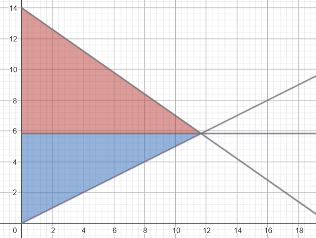
For the \(i\)-th brownie, its marginal benefit \(P\) is the intersection of the demand curve with the line \(Q = i\). What happens when this \(P\) is higher than the market equilibrium price, which we'll call \(P_m\)? Well, the customer buying that \(1\) brownie must be very happy: they were willing to pay \(P\) for it, but they only had to pay \(P_m\). We call this difference, \(P - P_m\), the consumer surplus.
But customers are discrete, fleshy meatbags. We want to– you get the point. Something something calculus; it's the area of the (triangular-ish) region above the equilibrium price and below the demand curve.
Unsurprisingly, we also have producer surplus. That'd be the area of the (triangular-ish) region below the equilibrium price and above the supply curve.
The sum of these is known appropriately as the total surplus.
Elasticity
How can we intuitively compare different markets with each other? After all, the boys sell other baked good(s), like apple pies, and those might be produced and consumed at wildly different prices or quantities.
One such metric we can use is elasticity. Consider some point on the demand curve. Here we'll just take the equilibrium price and quantity, \(P\) and \(Q\). The price elasticity of demand is the ratio between the percentage change of quantity demanded and the percentage change of price.
In symbols, this would look like:
Note the approximate symbol. Since \(\Delta P\) (and thus \(\Delta Q\)) is chosen somewhat arbitrarily, we might end up with slightly different values of \(\epsilon\). But of course, you already know by now that I'm a calculus zealot, so:
By definition, \(\epsilon\) depends on where on the demand curve you are. Again, here we're taking it at the market equilibrium, because, well, that's where markets tend to be anyway, right?
Also by definition, unless the market is incredibly cursed, \(\epsilon\) here must be negative. An increase in price results in a decrease in quantity demanded, after all. So by convention, we'll talk about its absolute value \(|\epsilon|\) instead.
You can find the elasticity of pretty much anything. Price elasticity of demand, price elasticity of supply, income elasticity of demand, cross-price elasticity of demand, whatever. Anything differentiable, most likely you can find its elasticity.
Elastic and inelastic demand
Let the total revenue \(TR\) be price times quantity, so \(TR = P \cdot Q\). Then, by the product rule:
Thus, we can conclude that:
-
If \(|\epsilon| > 1\) (so \(\epsilon < -1\)), then \(\frac{dTR}{dP} < 0\), which means increasing the price by a small amount results in a small decrease in total revenue. We call this elastic demand.
-
If \(|\epsilon| < 1\) (so \(\epsilon > -1\)), then \(\frac{dTR}{dP} > 0\), which means increasing the price by a small amount results in a small increase in total revenue. We call this inelastic demand.
-
If \(|\epsilon| = 1\), then the demand is unit-elastic. A small change in price (positive or negative) basically won't affect the total revenue.
Why those names? Well, returning to our baker boys, if their baked goods were inelastic, that means their customers are loyal. If they charged a little bit more, the customers would still happily buy their baked goods. On the other hand, if their baked goods were elastic, that means their customers are more flexible with their options. Charge us more for your brownies? Who cares, we'll just go somewhere else.
In particular, when the demand curve is a simple downward-sloping straight line, the quantity \(\frac{dQ}{dP}\) is constant, so at higher prices \(P\) (and thus lower quantities \(Q\)), \(|\epsilon|\) is higher, so the demand is more elastic. Likewise, for lower prices \(P\) (and thus higher quantities \(Q\)), the demand is more inelastic. This makes sense: I have been eating cheap Mixue ice creams for years now, and damn it, I would still eat them even if they charged \(50\) more cents per ice cream.
Some funny edge cases:
-
If \(|\epsilon| = 0\), that means the demand curve is really a straight vertical line. No matter how wildly you change the price, the quantity demanded will not change. We say the demand is perfectly inelastic.
-
If \(|\epsilon| = \infty\), that means the demand curve is really a straight horizontal line. Make the price a little bit higher, and people will riot and stop buying your product immediately. Make the price a little bit lower, and people will go crazy and buy until you run out. We say the demand is perfectly elastic.
Elastic and inelastic supply
Self-explanatory.
Price controls
Andy and Benny are well-mannered boys, but unfortunately, not all of their customers are.
There are brownie wrappers everywhere. The whole country is a mess.
It isn't long before President Peter knocks on their doors…
Price floor
President Peter respectfully (and understandably) complains about how his citizens are eating too many brownies, so he proposes an idea to the boys: set the minimum price of brownies to be above the market equilibrium. What happens to the world then?
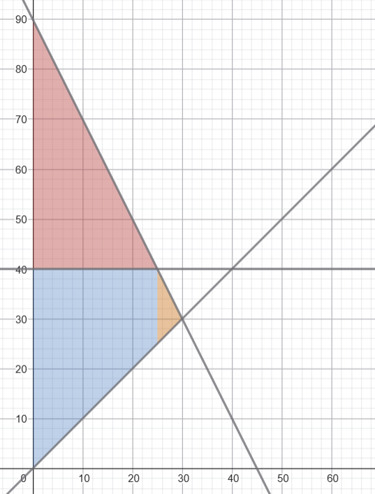
It's clear that the consumer surplus decreases. There's also a surplus of brownies in the market: at the current price level, the boys are willing to sell more brownies than the customers want to buy. The producer surplus may increase or decrease; it depends.
What's more important is the deadweight loss: the orange triangular bit that represents the loss in "economic welfare" (i.e., gainz) as a result. There are hungry customers who want to eat brownies, and the boys are willing to produce them. Sadly, for those hungry customers, the price they are willing to pay for a brownie is lower than the price floor, so they won't buy their precious brownies.
The boys are devastated. The customers are heartbroken. Everything sucks.
Price ceiling
President Peter quickly realizes his mistake and rushes to the boys' bakeries. As an act of forgiveness, he offers to set the maximum price of brownies to be below the market equilibrium.
The boys, not really thinking straight at this point, enthusiastically agree.
The next day, the boys quickly realize their blunder.
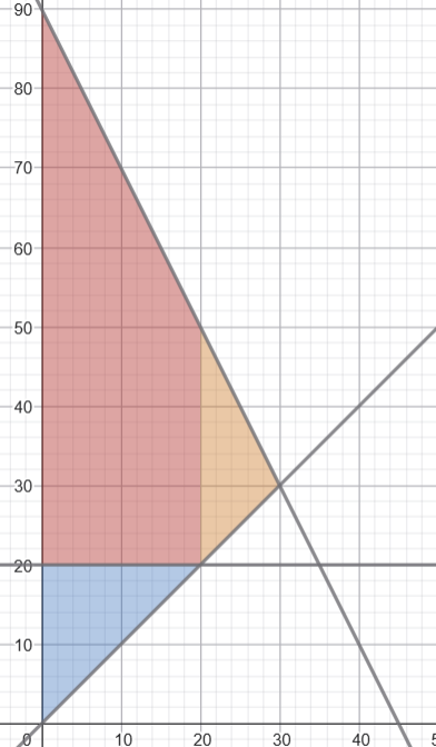
Now there is a shortage of brownies in the market: at the current price level, the customers are willing to buy more brownies than the boys want to produce. The producer surplus decreases; the consumer surplus could go either way.
There is still a deadweight loss.
The boys are in shambles.
Taxes
After several heated arguments civilized discussions with President Peter, the boys begrudgingly agree to have a tax \(T\) imposed on each brownie sold. If the customers are this frenzied over brownies, President Peter may as well seize the opportunity for the greater good: education, housing, infrastructure, one more private yacht for his collection, and so on.
Imposed on producers
Suppose the tax \(T\) is imposed on the boys: every year or so, the boys have to visit President Peter's office and hand him their hard-earned cash.
The demand curve does not change, since the customers are indifferent to the boys' misfortune. But what happens to the supply curve?
Recall that the supply curve really represents the marginal cost of producing each additional brownie. Since the boys have to pay \(T\) to President Peter for each brownie they sell, the whole supply curve shifts up by \(T\) as a result.
The new equilibrium quantity, \(Q_t\), must be less than the original market equilibrium, \(Q\). In particular, the corresponding point \((Q_t, P_c)\) on the demand curve and the corresponding point \((Q_t, P_p)\) on the old supply curve must satisfy:
Unsurprisingly, this implies:
Imposed on consumers
Next, suppose the tax \(T\) is imposed on the customers instead: every year or so, each individual customer must visit President Peter's office and (truthfully!) pay \(T\) for each brownie they bought throughout the period. The line is unimaginably long; you have no idea.
This time, the supply curve does not change: the boys can relax and not have to deal with President Peter for a short while. Now, the demand curve really represents how much the next customer is willing to pay the boys for the next brownie. Since each customer has the additional burden of paying \(T\) to President Peter for each brownie they buy, the price they're willing to pay the boys will decrease by \(T\). Thus, the demand curve shifts down by \(T\).
Again, we have \(Q_t < Q\), and the corresponding point \((Q_t, P_p)\) on the supply curve and the corresponding point \((Q_t, P_c)\) on the old demand curve must satisfy:
which implies:
…wait.
Relativity
So it turns out that it doesn't really matter who the tax is imposed on: the price \(P_c\) paid by the consumer and the price \(P_p\) received by the producer don't change, nor does the equilibrium quantity. The shifts in the curves may vary, but as long as the difference \(P_c - P_p\) (the wedge) is equal to \(T\), President Peter is happy. You can even imagine a convoluted scheme where the boys pay \(\frac{T}{2}\) for each brownie sold, and the customers pay \(\frac{T}{2}\) for each brownie bought.
What happens in the real world? As with all things, it depends. Sometimes taxes are remitted (or paid to the government) by companies, e.g., for retail goods. Sometimes taxes are remitted by individuals, e.g., for owning vehicles. And obviously, no one is knocking on the president's door; taxes are usually paid via a tax authority like the IRS.
That's cool and all, but in the end, who actually pays what?
Economic burden
The customers pay \(P_c\) for each brownie they buy, instead of the lower equilibrium price \(P\). Similarly, the boys receive \(P_p\) for each brownie they sell, instead of the higher equilibrium price \(P\).
We say that the consumers carry the burden of \(P_c - P\) per brownie, and the producers carry the burden of \(P - P_p\) per brownie.
Now, who carries the heavier burden? Here's a neat trick: we can directly compare the (absolute) elasticities of supply and demand at the market equilibrium. The \(\frac{P}{Q}\) terms (remember?) cancel out, because we're taking both at the same point. So essentially, we're just comparing the slopes of both curves. The curve whose slope is steeper (i.e., is more inelastic) corresponds to the side that bears the heavier burden.
Fundamental theorems of welfare economics
For this section, I think it's better to discretize everything. Assume there are no tax shenanigans.
The supply curve represents the marginal cost of producing the next brownie, and the demand curve represents how much the next customer is willing to pay for it.
So you can imagine a queue at the bakery where customers are ordered by how much they're willing to pay for their precious brownie.
When it's the \(i\)-th customer's turn, we look at the corresponding points on the supply and demand curves: \((i, P_p)\) and \((i, P_c)\), respectively. What that means is that the \(i\)-th customer is willing to pay at most \(P_c\) for the \(i\)-th brownie, and the boys are willing to receive at least \(P_p\) for the \(i\)-th brownie.
If \(P_c > P_p\), that's great news: the transaction is successful as long as the price falls between \(P_p\) and \(P_c\), and both sides will benefit from it. If \(P_c = P_p\), then both sides are indifferent; it doesn't really matter whether or not the transaction goes through. But if \(P_c < P_p\), then too bad, no transaction occurs because there is no price that both sides would agree on.
Now let \(Q\) be the equilibrium quantity in the market. We can see that all transactions before the \(Q\)-th brownie benefit both sides, and all transactions after the \(Q\)-th brownie do not. Thus, after \(Q\) brownies are sold, we are in a situation where "no one can be made better off without making someone else worse off". We describe such a situation as Pareto efficient.
The first fundamental theorem of welfare economics states that, under the (extremely) idealized conditions we've been working with so far, an equilibrium in a competitive market will be Pareto efficient.
Now, the first theorem does not make any guarantees about whether the resulting allocation of brownies is "fair". Cindy may well be allowed to cut in line multiple times, as long as she has the money to pay for her brownies. Surely the other customers would get upset.
President Peter proposes yet another idea. This Saturday, everyone will pay him a fixed tax (this is a type of lump-sum tax). Then, on Sunday, he will redistribute the accumulated taxes back to everyone in a way that's… "desirable".
The second fundamental theorem of welfare economics states that, given a "desirable" Pareto efficient situation, there exists an initial redistribution of resources (for example, through lump-sum taxes and transfers) such that, in the end, when everything has stabilized and the competitive market is in equilibrium again, we end up in exactly the situation that we desired.
So yes, as long as they're Pareto efficient, we can achieve outcomes where Cindy gets a lot of brownies, or perhaps outcomes where she gets none at all.
There is one big asterisk to all this, though. President Peter still has to decide what situation is "desirable". He could try asking each of his citizens to rank all the possible outcomes, but what if those rankings conflict with each other? After all, he knows that all Cindy would want is a bajillion brownies. This is a whole other story that we may or may not leave for another time.
Externalities
Let's come back to those litterbug customers. They are rude, annoying, and they litter brownie wrappers everywhere. President Peter's Robot Cleaners™ have to work much harder to clean up the whole mess.
Now, Andy and Benny don't have to pay for the Robot Cleaners™ to work harder. For all they care, the costs are coming from President Peter's pocket anyway. But surely President Peter is unhappy: he is incurring a cost that isn't accounted for in the cost of producing or consuming a brownie. The customers don't have to pay for this cost, nor do the boys.
This is known as an externality. In particular, it's a negative externality, because President Peter has to pay more for the Robot Cleaners™ as a result of the boys' brownie antics.
As we've seen, one way to deal with negative externalities is to impose a tax on producers or consumers to reflect this external cost, creating an artificial shift in the corresponding curve. This decreases the equilibrium quantity, and President Peter is more than happy to do so.
On the other hand, there are positive externalities: benefits received as a result of the actions of another party. The classic example is vaccines: getting vaccinated protects yourself, but it can also help protect others from harmful viruses. To encourage vaccinations, governments can offer subsidies: decrease the cost of getting vaccinated to increase the equilibrium quantity.
All the costs
There are a bunch of cost curves for a bunch of things. Here we'll always take the \(x\)-axis to represent how many brownies the boys consider producing in a day, and the \(y\)-axis to represent some measure of cost at that level of production.
Fixed Cost
No matter how many brownies the boys produce, they'll still have to pay the same amount of rent each day. This is known as the fixed cost (\(FC\)).
Clearly, the \(FC\) curve is just a straight horizontal line.
Variable Cost
As we all know by now, the cost of producing brownies (ignoring fixed costs) changes depending on how many brownies are produced. This is known as the variable cost (\(VC\)).
The \(VC\) generally increases, because, well, producing more stuff costs more.
Total Cost
It's just fixed cost plus variable cost. \(TC = FC + VC\).
Marginal Cost
As before, the marginal cost (\(MC\)) is the cost of producing \(1\) additional brownie.
The \(MC\) is the derivative of the \(TC\), but it's also the derivative of the \(VC\), because that's how math works. A nice consequence is that the variable cost can be thought of as the sum of the marginal costs of each brownie produced so far.
The U-shape
Many sections ago, I wrote:
As we've seen with the PPFs, the more brownies the boys produce, the more apple pies they have to give up per \(1\) brownie. This is generally true not just relative to apple pies: the more brownies you produce, the marginal cost (say, in dollars) of producing \(1\) additional brownie eventually increases.
but then I made this dubious assumption:
Here we'll just assume it always increases.
Now, a strictly increasing marginal cost is possible, but not as common. We should also account for how the robot bakers work with each other.
At the start, only the robots that are (relatively) very good at producing brownies are on brownie duty. This is fine and all, but the problem is that there aren't enough robots to split up the work efficiently: they have to run around between counters and ovens, which is a huge waste of time. Eventually, though, as more brownies are produced, more robots are allowed on brownie duty, and the bakery enters a steadier rhythm of producing brownies.
This results in the U-shape economists know and love: the \(MC\) initially declines when the bakery is operating at too low an output level, then starts rising again once the specialization benefits run out and the boys have to use robots that are (relatively) less good at producing brownies.
Average Fixed Cost
Fixed cost divided by quantity produced. \(AFC = \frac{FC}{Q}\).
Naturally, the \(AFC\) is decreasing, because the \(FC\) is constant.
Average Variable Cost
Variable cost divided by quantity produced. \(AVC = \frac{VC}{Q}\).
Usually, the \(AVC\) is also "U-shaped". The intuition is similar to why the \(MC\) is U-shaped.
However, it's been a while since we've done some actual mathematics, so…
This has some pretty neat consequences:
- If \(MC > AVC\), then \(\frac{d}{dQ}\left(AVC\right) > 0\), so \(AVC\) is increasing.
- If \(MC < AVC\), then \(\frac{d}{dQ}\left(AVC\right) < 0\), so \(AVC\) is decreasing.
- If \(MC = AVC\), then \(\frac{d}{dQ}\left(AVC\right) = 0\), so \(AVC\) is at a stationary point, which is the minimum, assuming the \(AVC\) really is U-shaped.
Or, in English:
- If the \(MC\) is currently higher than the \(AVC\), we should expect the \(AVC\) to increase.
- If the \(MC\) is currently lower than the \(AVC\), we should expect the \(AVC\) to decrease.
- The \(MC\) curve intersects the \(AVC\) curve at the \(AVC\) curve's lowest point.
Average Total Cost
Total cost divided by quantity produced. \(ATC = \frac{TC}{Q}\).
By the power of mathematics, the same properties of \(AVC\) also apply to \(ATC\):
Perfect competition
At last, we are ready to (more or less) characterize what we've been talking about thus far.
Andy and Benny are merely two boys among countless bakers scattered throughout the country. They have little to no effect on the market price: they can't just charge twice as much for their brownies and expect everyone else to do the same.
Maybe in a few decades, they could dominate the brownie market and form an oligopoly with a few other great bakers, or take over the whole thing and form one big monopoly. But for now, the boys are humble price-takers: it's best for them to sell their brownies at the market price.
Strangely enough, Andy and Benny have been sharing the exact same brownie recipe for months now, and no one has noticed. Their loyal customers still think they've been at each other's throats for years. Maybe they should announce their relationship soon?
Regardless, their brownies are homogeneous: they are perfect substitutes for each other, and the quality of the good does not vary between different suppliers.
President Peter is annoying sometimes, but he's still kind-hearted at the end of the day. Public transport is free for everyone, so customers don't have to spend money to reach the boys' bakeries; they only have to pay for each brownie itself. Similarly, the boys don't have to pay anything extra either.
We say the market has no transaction costs: buyers and sellers do not incur additional costs when participating in a transaction. Also, there are no barriers to entry and no barriers to exit: Andy and Benny can freely open or close their bakery without any restrictions.
Lastly, there is perfect information: Andy and Benny are up to date on the latest news on brownie prices across the country, and so are their customers.
These conditions (and many more I'm not going to cover because we'd be here all day) make up what is known as a perfectly competitive market.
Marginal revenue
The marginal revenue \(MR\) is the revenue earned by selling \(1\) more brownie, or mathematically, the derivative of the total revenue \(TR\) with respect to the quantity \(Q\):
Now, it's worth noting that the elasticity (and hence \(MR\)) can be taken relative to the entire brownie market as a whole, or relative to the boys in particular. Here, we're focusing on the latter.
Assuming a perfectly competitive market, Andy and Benny obviously shouldn't charge more than the market price, because then no one would go to their bakery. They shouldn't charge less than the market price either, because then they'd just be making less money.
Sound familiar? The boys' individual demand curve is perfectly elastic. This means \(|\epsilon| = \infty\), so the above just simplifies to:
In other words, no matter how many brownies the boys sell, they will always earn a marginal revenue of \(P\) for each additional brownie.
Profit
Equals total revenue minus total cost. \(\Pi = TR - TC = Q(P - ATC)\).
Maximizing profit
Recall that the \(MC\) initially declines, then rises again. Andy and Benny should produce brownies until they reach the unique2 quantity \(Q^*\) where \(MC(Q^*) = P\):
- For \(Q < Q^*\), we have \(MC(Q) < P\), so producing another brownie increases profit, which means they should keep producing brownies.
- For \(Q > Q^*\), we have \(MC(Q) > P\), so producing another brownie decreases profit, which means they should stop producing brownies.
In English, they should continue producing brownies until the marginal cost of producing \(1\) more brownie exceeds the market price.
What can we say about the profit \(\Pi\)? For that, we'll compare \(P\) with the break-even price \(P_{be}\), the minimum value on the \(ATC\) curve:
- If \(P < P_{be}\) (i.e., \(MC(Q^*) < P_{be}\)), then we are below the \(ATC\) curve, so \(\Pi\) is negative.
- If \(P > P_{be}\) (i.e., \(MC(Q^*) > P_{be}\)), then we are above the \(ATC\) curve, so \(\Pi\) is positive.
- If \(P = P_{be}\) (i.e., \(MC(Q^*) = P_{be}\)), then we are on the \(ATC\) curve, so \(\Pi\) is zero.
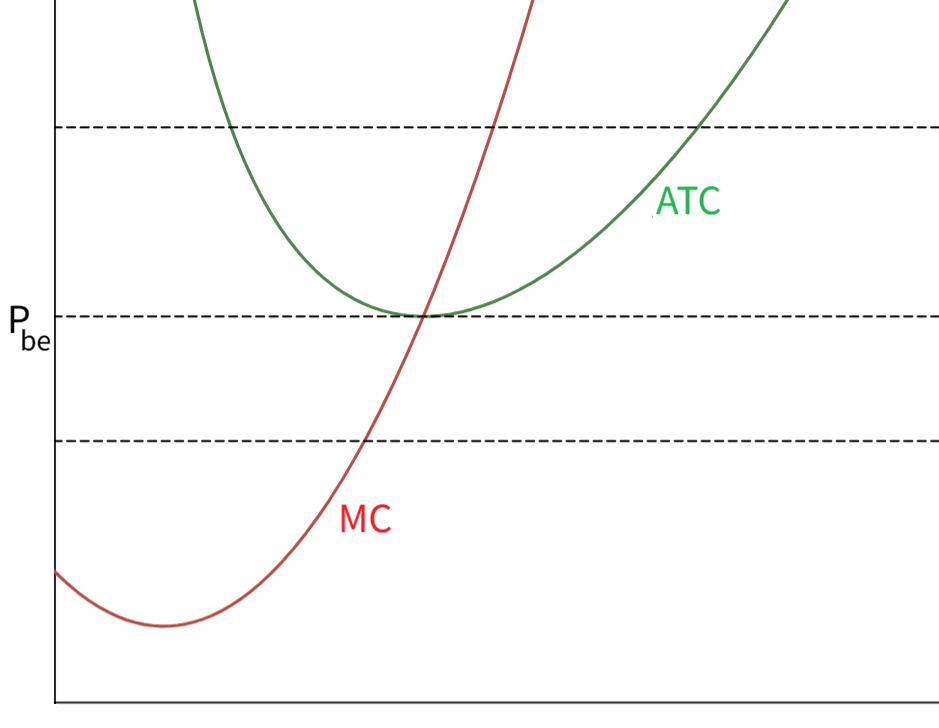
Note that all these derivations implicitly assume that Andy and Benny have already started producing brownies. But what if the best course of action for them is to not produce anything?
Short run and long run
Clearly, if \(P > P_{be}\), then the boys should produce brownies, because they'd be making a profit. But what about \(P \leq P_{be}\)? Does that mean the boys shouldn't produce any brownies at all, because they'd be making a loss?
Well, not necessarily. After all, the boys still have to pay rent, brownies or not. So if the revenue they'd earn is more than the variable cost, then they can at least use that difference to cover part of their rent. Hey, something is better than nothing, right?
In other words, if \(TR - VC = Q(P - AVC)\) is positive, then it's still worth producing brownies. If the difference is negative, then they should temporarily close their brownie operations for now.
We can do something similar to before. This time, we'll compare \(P\) with the shutdown price \(P_{sd}\), the minimum value of the \(AVC\) curve:
- If \(P < P_{sd}\), then we are below the \(AVC\) curve, so the boys should not produce brownies.
- If \(P > P_{sd}\), then we are above the \(AVC\) curve, so the boys should produce brownies.
- If \(P = P_{sd}\), then we are on the \(AVC\) curve, so the boys are indifferent.
Ultimately, though, this is only for the short run. In the long run, fixed costs are no longer fixed: the boys are planning to buy a house together sometime in the future, anyway. So there's really no point in them maintaining their bakeries when \(P < P_{be}\). If that happens, they'll just run off into the sunset together.
-
I know convergence subtly implies they were divergent to begin with, but that's not really accurate. Of course, things still shift around and eventually settle after significant changes in a market, but markets are usually stable most of the time. You get what I mean. ↩
-
Please ignore the funny edge cases where there are \(0\) or \(2\) intersections. ↩